Nathan Blake

Explainable AI is any process in which we try to identify which features a model used in making a particular prediction. But what happens when we want to explain something that is defined by the absence of features? A model may learn that certain pixel characteristics are associated with a brain tumour, and an XAI tool may then pick those out in a given image. But what features does it associate with no tumour? This is a subtle problem, and one that needs addressing if various regulatory and clinical demands for applied AI are to be met. We have developed an Algorithm called NITO which begins to address this issue. (Available here.)

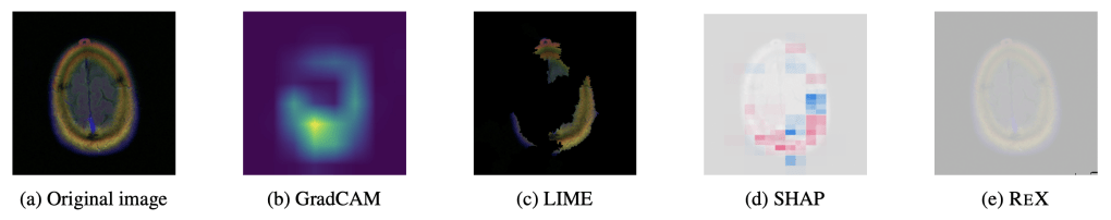
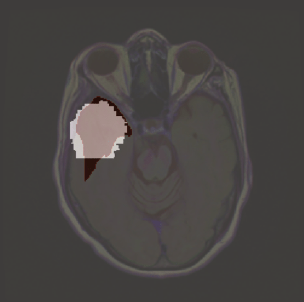
‘Explaining’ the absence of disease. Common XAI tools will produce heatmaps, ostensibly locating to where there is no tumour. But this entire brain slice is absent of any tumour. Arguably, ReX has the most ‘informative’ landscape as it is utterly uninformative (i.e. nearly completely flat), though this is not clinically useful.

NITO

NITO, Yiddish for ‘not there’ or ‘is not present’, uses a definition of an explanation from actual causality. In this framework, an explanation is (roughly), a minimal subset of features (pixels in this case) which are sufficient for the model to return its original classification. It’s minimal in the sense that removing any subset of pixels will result in the set no longer being classified as a tumour. NITO needs a definition of an explanation as it will use this to show that no such explanation can exist in a ‘normal’ image

First, NITO constructs a subset of all slices corresponding to a particular location in all images, called K,. Imagine each brain scan as a 3D object, each slice then corresponds to a different depth. K is the set of all the same anatomical slices in the entire dataset. (Note, in this case the model is still trained on 2D slices). From this, we find the smallest explanation. We use ReX to do this – due to its approximate minimality, its explanations are usually smaller than the tumour itself.

With this smallest explanation in K, NITO then constructs an absence grid. This is a grid of collections of pixels, with the radius and density of the grid adjusted so that it will not allow the smallest explanation to fit into it.

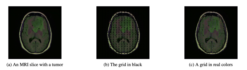
It is important that the grid values themselves do not cause the classification of a tumour. This might be some healthy value or neutral value interpolation (like black or grey – which are not a natural colour in these images – which although not healthy, neither is it diseased).

We then calculate the β-goodness of the fit. This is the proportion of slices in K which give a ‘no tumour’ prediction after the grid is imposed.Ideally we’d like this to be 1, which would indicate (for this model and dataset) that the grid ensures a ‘no tumour’. For lower values of β we may be more circumspect of the results – quite what is a good threshold has yet to be determined, though will almost certainly be case and use dependent, and require careful calibration with clinical partners. There are more nuanced ways of calculating β as a probability explored in the paper.

Clinical Use

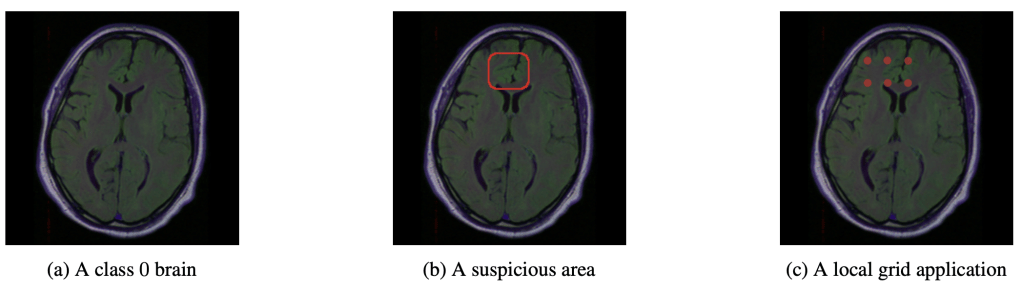
NITO will allow a clinician to ask the question of why a model predicts the absence of a tumour in a particular image. For example, we can imagine a scenario in which an AI system is used to triage scans into high or low priority, alongside a radiologist ( this is a realistic vision of future clinical AI use – sorry Hinton, but it’s still going to be a long time before radiologists are replaced by AI). The radiologist may be inspecting the low priority predictions when they notice a suspicious area. Using NITO, they may inspect the region to show why the model ‘thinks’ no lesion can exist in that locale. The radiologist may well disagree. It might be even more suspicious if the β-goodness is low for this slice location. But at leasst the clinician would have some idea why, from the models perspective, a tumour cannot fit inside the imposed grid.

Assumptions

NITO assumes the locality of explanations: that the cause of a model giving a classification for a given image is to be found in one or more discrete locations. There may be several such locations. This assumption works for things like solid tumours, but fails when causal features are dispersed throughout the image (such as may be the case with Alzheimer’s disease).

Nito also assumes pixel independence. We know this is not strictly true, but empirically we get reasonable results. anyway. In large part, this is due to the relative homogeneity of medical images as compared to general images. Still, this could be an area of improvement, if we can get around the problem of exponentially large search spaces.

Crucially for clinical applications, the method is only as good as the dataset it was trained upon. If the dataset does not represent the distribution of possible tumours (especially those of smaller size), then it is quite possible that NITO will construct an incongruent absence grid – it may be too sparse. Of course, if your dataset is not actually representative then you have much bigger problems for any real clinical deployments.

I’ll be presenting this at the UAI 2025 conference, so come and find me if you’re there.